Adjusting to Real Dollars in R
January 08, 2018
January 08, 2018
Using R to adjust a time series of dollar values for inflation:
This post is the first of several that I have planned that focus on some of the simple tasks that I have been using R to help with. Although this task might be relatively simple, in subsequent articles I’ll continue to expand in some tasks that are longer and more specific.
I’ve been using R a lot to wrangle data. R scripts are useful if you find yourself performing the exact same task across different projects and would like to accomplish your goal by just reading in a file and clicking ‘run.’ Typically I am working with similar datasets, such as the Census, travel, home sales, and PUMS records.
I’ve been focusing a lot on housing affordability trends and developing forecasts in my recent work. To help do this, part of my research has focused a lot on working with home sales data an available time-series of housing costs. For most cities and localities, if you go to the county assessor’s office you can often get a full dataset of all home sales in a region over a period of time. Sometimes you can download it directly from the website, and other times you’ll need to do a little more research, such as contacting someone at the assessor’s office. Either way, I’ve found that you can almost always find it after a little digging around and its a great resource to have.
Whenever I work with this dataset, the first thing I need to do is to quickly adjust all of the dollar figures for inflation, usually to 2016 or 2017 real dollars. The R package, quantmod, help you download data from the consumer price index.
The code below will grab data by month, but you can adjust it for yearly, or even daily values.
##################################################


#Adjusting all dollars using consumer price index


##################################################

library("quantmod")


#Get CPI Data from online using GetSymbols which is a part of the quantmod package
getSymbols("CPIAUCSL", src='FRED')
set.seed(1)

#You'll have to adjust this for different date ranges by changing the from date and length.out
#Look up the documentation on xts() as well to get a better idea of the variables used here.

p <- xts(rnorm(224, mean=10, sd=3), seq(from=as.Date('1997-01-02'), by='months', length.out=224))
colnames(p) <- "price"


#Get ratio of index to a base year.
avg.cpi <- apply.monthly(CPIAUCSL, mean)
cf <- avg.cpi/as.numeric(avg.cpi['2017'])#using 2017 as the base year


#Join to original sales data
adjRate <- data.frame(date=index(cf), coredata(cf))
rm(p, cf, avg.cpi, CPIAUCSL)
adjRate$key <- format(as.Date(adjRate$date), "%Y-%m")
There you go. Now you can merge this into a data file and divide the prices by the adjusted rate. This will give you the real values in 2017 dollars. Just for reference, I’ll add a little an example below where I merged this into an existing dataset.
Seattle$key <- format(as.Date(Seattle$DocumentDa), "%Y-%m")
Seattle <- merge(Seattle, adjRate,by="key", all=FALSE)

rm(adjRate)


#Adjust Prices according to the rates.

Seattle$realSalePrice <- Seattle$SalePrice / Seattle$CPIAUCSL
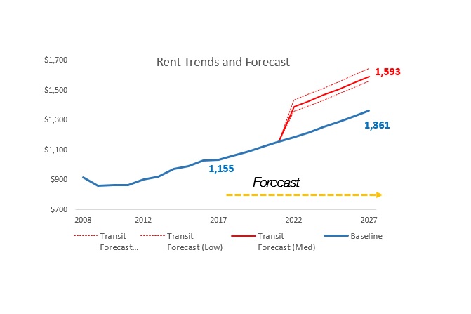
Once you have something like this on hand, I’ve found that it is pretty useful in various tasks. For example, I also find myself grabbing this code in other instances whenever calculate the combined annual growth rate in rising rents from sources such as CoStar. Not accounting for inflation can make the increases seem huuuuuuuge, when in fact they may be relatively modest after adjusting for inflation.
The code posted above can also be found on my GutHub account here.
Next post: Using R’s ACS api package to grab census data.