Fiscal Impact Analysis at SGA
December 05, 2017
December 05, 2017
A brief overview of the fiscal impact analyses that I perform as a data analyst at Smart Growth America.
I’ve been working as a data analyst for almost a year now at a DC-based non-profit, Smart Growth America (SGA). For the most part we provide technical assistance and facilitate workshops for communities around the country that promoting land-use policies that lead to healthier, walkable, mixed-used communities.
One of the tools that we use to evaluate the impact of different land-use policies is a fiscal impact analysis. A fiscal impact analysis looks at the costs of development, and calculates the revenues generated with the difference being the ‘impact.’ Typically, lower density development leads to a negative impact, and the costs for infrastructure need to be collected somewhere along the line to compensate for this gap. However, with a high enough density the costs of building roads, schools, etc. are offset by the concentration of revenues and the impact is positive, a revenue for the community.
Our methodology at SGA uses observations of existing development patterns gathered from GIS, and then runs them through a regression to identify the trend between population density and infrastructure. (The formula of the fitted regression line is used to estimate costs for a given population density.) Based on these observations, we can calculate the cost of new development that matches a pattern similar to the existing observations. Usually this analysis is used to compare the impact of various density alternatives for development.
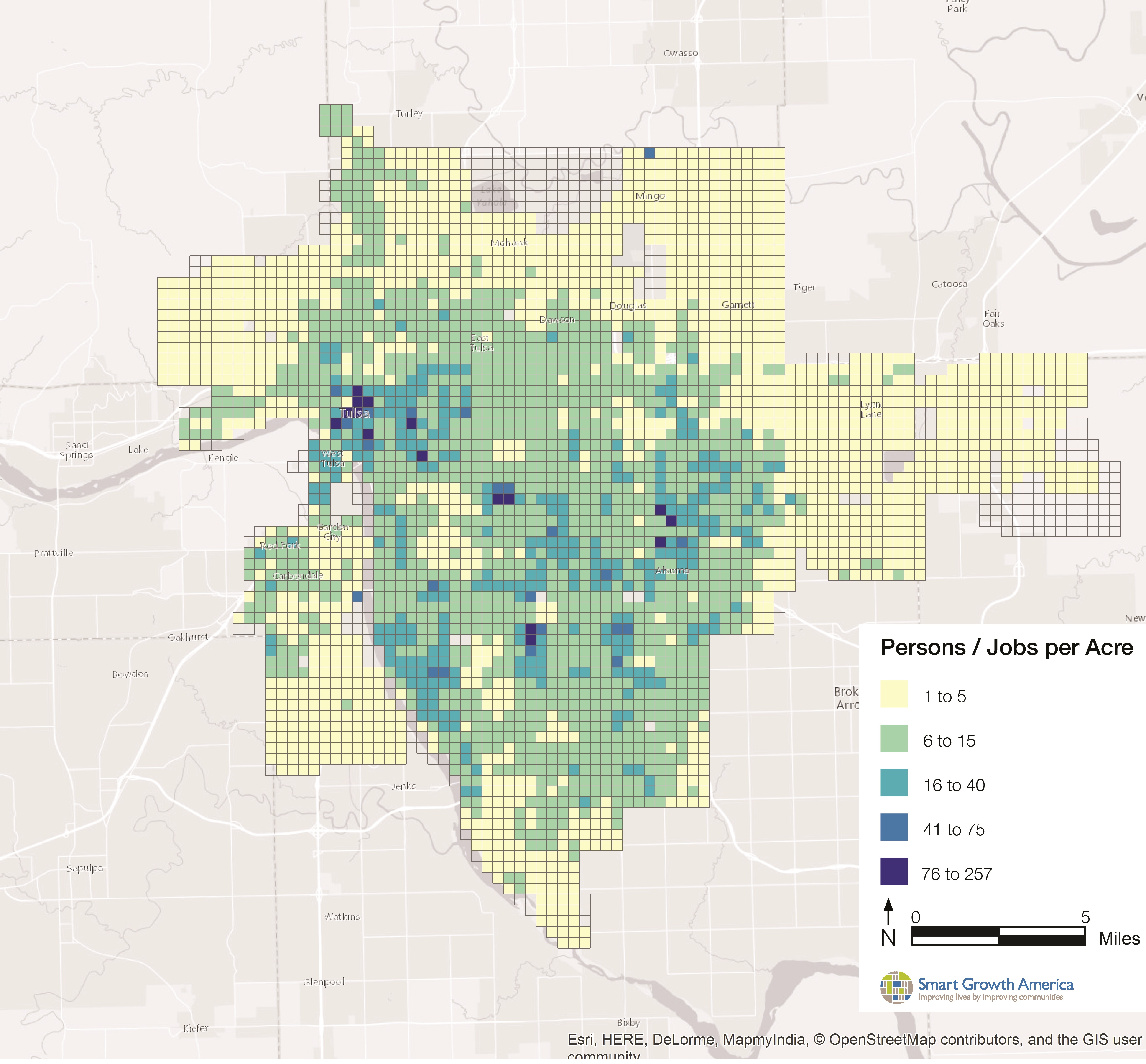
The first step of the process involves gathering shapefiles that pertain to population (Census Blocks), employment (again: from the Census), and infrastructure items such as roads, sidewalks, sewers, water, etc. We divide each of these components into 40-acre grid cells for comparison. Dividing observations into equal grid cells is a process similar to research methods used in other studies such as this Report from the National Trust for Historic Preservation: “Older, Smaller, Better.”
Dividing up census blocks, and other shapefiles such as roads can be done in GIS using intersect and a number of other tools in succession. This process is almost always the same, so to save time I created a custom ArcMap toolbox by writing a few python scripts, which I have also shared via GitHub. Below is an example of population + employment density observations per 40-acre grid cells.
Population and Employment Density Observations
(40-acre grid cells)
The next step of the process is to create a bivariate regression for each infrastructure item and compare the observed amount of infrastructure per capita for each level of density. The typical result found is an exponential relationship between population density and infrastructure per capita. (The degree to which this fits along a regression line does vary from place to place.)
Below is a sample of the regression generated measuring road area per capita by population density. At higher densities, there are more people sharing each square foot of road. A lower densities, that same square foot of road is shared by fewer people (and thereby there are less tax revenues to support the construction and maintenance.)
Scatter Plot of Bivariate Regression for Road Area from R
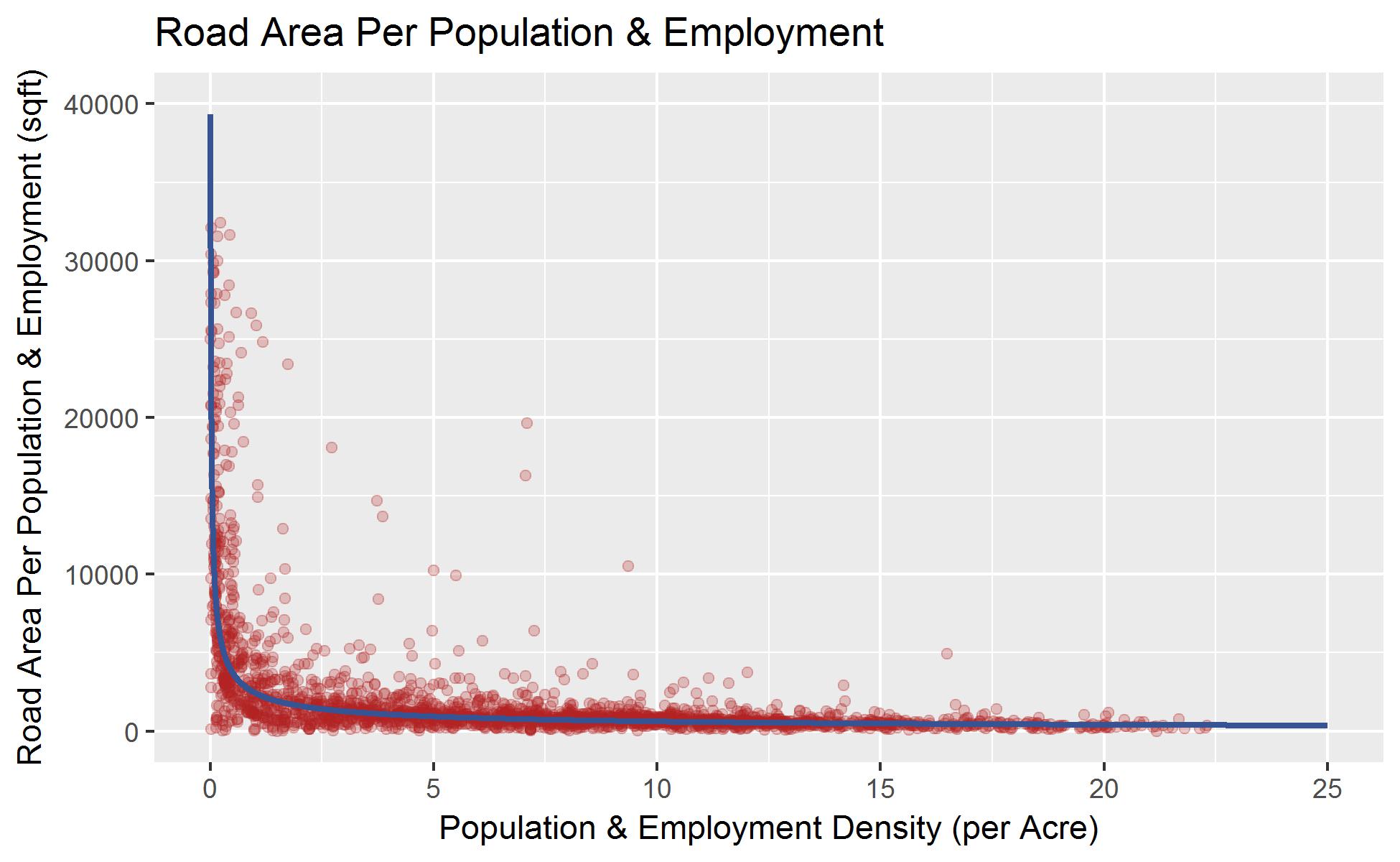
Just like with the grid cells, the process of creating regressions for each place is very similar. Again, to save time and document the process I’ve created scripts in R that will work through the input files generated from my custom ArcMap toolbox.
The final step is to calculate the costs for each infrastructure item, using the formula of the fitted regression and compare these to the projected tax revenues that the development should generate. The bottom line of a fiscal impact analysis often looks like the bar graph below.
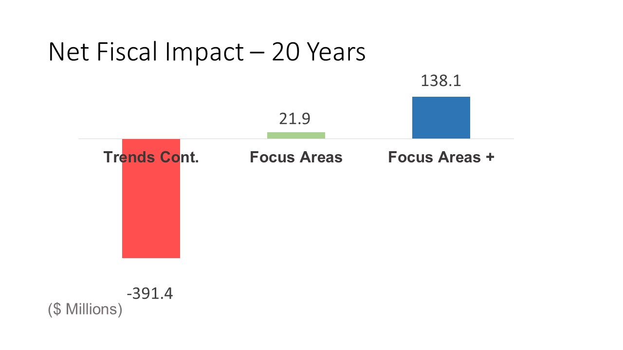
In the example above, the Trends cont. scenario contained a mostly suburban development pattern with low density levels such as 3 households per acre. The Focus Areas, and Focus Areas + Scenarios, were higher density, mixed-use developments that had densities such as 10 or 12 households per acre. This analysis is good tool for providing a comparison of how the change in density can also change the bottom line in terms of infrastructure costs. It also provides a good opportunity to combine GIS and statistics for use in policy analysis.
If you would like to seem some of the final reports released from Smart Growth America using this methodology, they can be found on their website HERE