Using R's ACS Package
March 23, 2018
March 23, 2018
In my last post I walked through some of the packages in R that make it really easy to grab and update data for a project. One of my favorites shortcuts is using the “ACS” package in R.
Now lets say you’ve filtered a select group of Census Tracts and need one or two pieces of information just for those tracts. This is especially tedious if you needed this data for a large number, like 40,000 tracts. In my case, I am often studying the profile of market rate rental units and their affordability in a neighborhood. In each study, I’ll need to gather and summarize data from just a few fields for these tracts. (At the end of this article I have a link to a more robust example of code and a sample input file to go with it.)
Saving time here will let me focus on other tasks that may be helpful to add for an area. For example, in some situations only a portion of some of the census tracts would fall within a neighborhood or other boundary and in those cases I might expand upon my existing code by adding a few lines to multiply the results from the ACS against a ratio.
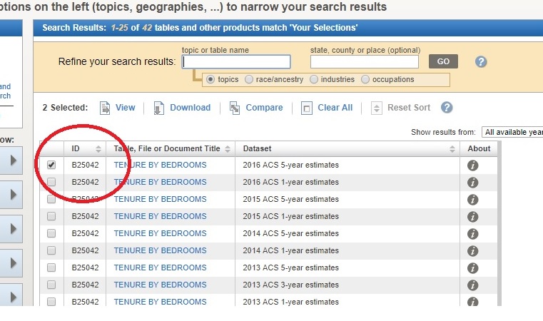
To grab the data you just need to identify a few pieces of information such as the year, and the name of the table which can be found on the census website, such as in the photo below. (The circled table number is what R will fetch for your selected geography.)
This package is great and can save you from digging through CSV’s from American Fact Finder, where you are trimming out just the columns and rows needed over and over. Below is a sample that takes an input file of census tracts, grabs specific data, and sums that data for the area.
# ==========================
# clear workspace
rm(list=ls())
dev.off()

library(easypackages)
libraries("acs", "foreign", "dplyr", "tidyr")

###########################################################################################

###########################################################################################

###########################################################################################


setwd("D:/Users/SGA1/Desktop")

#Replace this with the location of your tract shapefile's DBF
dat = read.dbf("INPUT_Study_Area_Tract_Intersected.dbf",as.is = TRUE)


##  ##  ##  ##

api.key.install(key="93e49ee8faa35fcf7a0f4b1f55c9228aa88d6cac")

##  ##  ##  ##

# ACS requires a geo object for its search.
# Be careful that FIPS loaded as character, with the following"
# 2 digit state, 3 digit county, 6 digit tract

geo<-geo.make(state  = as.integer(as.list(dat$STATEFP10)),
              county = as.integer(as.list(dat$COUNTYFP10)),
              tract  = as.integer(as.list(dat$TRACTCE10)))


#Fetch data.
ACS_Rental_Units<-acs.fetch(endyear = 2015, span = 5, geography = geo,
                        table.number = "B25042", col.names = "pretty")
attr(ACS_Rental_Units, "acs.colnames")


#Convert from ACS object to a normal data frame.
ACS_Rental_Units <- data.frame(ACS_Rental_Units@geography, ACS_Rental_Units@estimate)


#Subsetting the dataset to just the fields that I need and renaming them.
ACS_Rental_Units <- ACS_Rental_Units[13:19]
colnames(ACS_Rental_Units) <- c("Units", "Studios", "1_BR", "2_BR", "3_BR", "4_BR", "5_BR")


#  Totaling the ACS data and changing to wide format with gather.
ACS_Rental_Units <- ACS_Rental_Units %>% summarise_each(funs(sum))
ACS_Rental_Units  <- gather(ACS_Rental_Units)
rownames(ACS_Rental_Units) <- ACS_Rental_Units[,1]

ACS_Rental_Units   <- spread(ACS_Rental_Units , key = key, value = value)
I have a longer sample of code that actually grabs and totals data from three different tables in the ACS and handles each slightly differently and exports them into a three-tabbed excel spreadsheet on my GitHub account HERE. I’ve also included an input file that you can use to run it. All you should need is R Studio with all the necessary packages installed to try it out (and adjust the line to set the workspace to your own desktop or wherever).
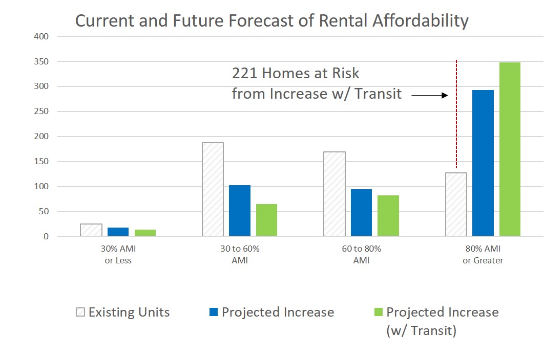
This profile of market rate rental housing was a small piece of a much bigger project that profiled the existing rental market and projected changes in affordability which I hope to cover later in several blog posts. Image below is a preview of the end result of this process where I was able to show the existing profile of affordability against two different projections for the future.